Learning Tomography: Simple Back-Projection

The simple back-projection is one of the most popular algorithm used to reconstruct an object from a series of projections. In this post, we'll study how to reconstruct a 2D image from 1D-projections.

1- Our data: A series of 1D-projections

In this example, we plan to compute a 2D-reconstruction from the series of 1D-projections shown in Fig.1.

Fig.1: Series of 1D-projections. This image is called a 'sinogram'. The top row corresponds to a projection calculated from a 0° direction and the last one to 179°.

Just few words on the image of Fig. 1, this is a collection of 180 1D-projections (Fig.2). The first row (top, y=0 ) was calculated from a 2D-image projected along a vertical direction (this is the 0° direction). Then, the other rows correspond respectively to projections calculated for 1, 2, 3, 4, ... up to 179°.

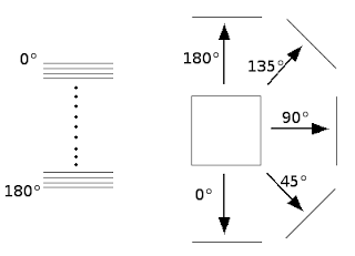
Fig.2: The sinogram is a collection of 1D-projections stored from top to bottom where the Y-coordinates correspond to their projection directions (here, expressed in degrees).

 Note: The scheme of Fig.2 isn't truly correct, the 180° 1D-projection isn't stored in the sinogram. We stop before 180°.

2- One back-projection by hand

To understand the principle of the algorithm presented in the next section, the best to do is calculating one back-projection interactively.

Step #1: Extract one row of the sinogram by selecting a rectangular area of 1 pixel high (Tool #1) as shown in Fig. 3A. Then duplicate it with the Image > Duplicate... command.
Step #2: A back-projection corresponds to the inverse transform of a projection (see previous post). Thus, in that case, converting a 1D-projection into a 2D image is simply done by resizing our 1D-projection to a square image using Edit > Adjust > Size.... We choose as parameters a height (equal to the 1D-projection width) of 256 and No (option None) Interpolation scheme (the fastest way).
Step #3: Rotation of the back-projection. In this example, I chose a row at Y=56. Then, I have to apply a rotation of -56 (the opposite of the original projection direction). This is done with Image > Transform > Rotate... (uncheck the 'Enlarge Image to Fit Result' option).

Fig.3: Steps to calculate a back-projection.

3- The script

This script is written in JavaScript because it's a little bit simpler and faster.

The first part of the script allows to get information about the sinogram to compute the angle step. Here, I assume that the angular coverage is 180°.
Then, the main loop computes a back-projection for each row composing the sinogram. The result is stored in a stack to see the various back-projections.

Note: The use of a stack is only for educational purpose, but isn't necessary in a normal reconstruction.

+++ IJ snippet: backProj.js +++ +++ End of IJ snippet +++

4- And now .... the reconstruction

Here is an example of what you can get with the script (Fig.4). Each slice of the stack is a back-projection correctly oriented to take into account the direction of projection.

Fig. 4: Several slices extracted from the final stack after execution of the script.

 The final step consists of adding all of the 180 back-projections. To have a good precision, we have to convert our stack in 32-bits. The addition is done with Image > Stacks > Z Project... command by selecting the 'Sum Slices' as Projection Type. Et Voilà.

Fig. 5: Result of the 2D-reconstruction obtained by averaging the images of the previous stack. Normalize the image to get a better contrast.

I must admit that the result is a little bit disappointing ... even though Lena is recognizable, the 2D reconstruction appears blurred.
Anyway, with this first approach, we were able to compute a 2D-reconstruction from a series of 1D-projections.
In a next post, we'll see how to improve our algorithm with the weighted back-projection.

Other crazybiocomputing posts

Further readings are available in ...

• Learning Tomography Series  [Link]
• Image Processing TOC [Link]