Exploring Gradient Direction

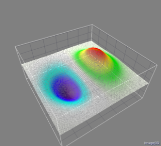
When working with gradient (for edge detection), it's rather interesting to visualize its orientation by drawing arrows and that's a good opportunity to try my previously published function drawArrow(...) [see post].


1- Computing gradient direction

Fig.1: Test image

If we look at the test image of Fig. 1 [see post] in 3D using the Plugins > 3D > Interactive 3D Surface Plot tool as shown in Fig.2, the 'landscape' is composed of a hole (cold colors: dark blue) and a hill (warm colors: yellow and red). The gradient corresponds to the transition of landscape in the image. The central steep part (from the hole to the hill) corresponds to the largest gradient whereas the flat (white) mesh has no variation.

Fig.2: Surface plot of test image. Heights (pixel values) are colored with the thermal LUT.

In mathematics, a gradient corresponds to the first derivative of a function (here, a 2D function: the image) and is defined in 2D by:

∇I(x,y) = (∂I / ∂x).i + (∂I / ∂y).j

Thus, a gradient can be decomposed in X- and Y-gradients yielding coordinates of vectors describing the orientation and direction of the 2D gradient.

The X- and Y- gradients are calculated by convolution with two Sobel 1D-kernels  respectively equal to:

Convolving these two kernels with the test image yield the images of Fig. 2A, and 2B. Each pixel value corresponds to the X- (and Y-) coordinates of the gradient vectors. Additionally, it's interesting to compute their norms √(Gx² + Gy²) to highlight the fast variations (transitions) of pixel values.

Fig.2: X-, Y-, and norm gradients of test image in Fig.1

The following lines allow the computation of the various images of gradient:

// X-Gradient
run("Duplicate...", "title=gradient_Gx");
run("Convolve...", "text1=[-1 0 1\n] normalize");
run("Duplicate...", "title=Gx2");run("Square");
// Y-gradient
selectWindow(in);
run("Duplicate...", "title=gradient_Gy");
run("Convolve...", "text1=-1\n0\n1\n normalize");
run("Duplicate...", "title=Gy2");run("Square");
// Gradient Norm
imageCalculator("Add create", "Gx2","Gy2");
rename("gradient_norm");run("Square Root");
getStatistics(area,mean,min,max);
run("Enhance Contrast", "saturated=0 normalize");

2- Visualizing gradient direction

Converting the pixels values in vectors (arrows) is done in a larger image (2x the original size; e.g. 256 x 2 = 512). Moreover, due to the arrow size of 16 pixels, only  256/16 pixels per line are drawn as arrows to avoid overlaps.

Here is the result...

Fig.3: Direction of the gradient calculated from the X- and Y-gradients of Fig. 2. The length of arrow corresponds to the vector norm.

And the script is composed of three parts:

• Lines 10-23: Computation of X-, Y-, and norm gradient images.
• Lines 27-39: Core of the script. Drawing of arrows by calling the function drawArrow(...).
• Lines 40-47: All the temporary images and the final arrows image are stacked.

+++ IJ snippet +++ +++ end of IJ snippet +++

3- Links

Example inspired by Matlab numerical gradient [Link]